Data Modelling and Analysis

Data Modelling and Analysis¶

Welcome to the fourth and last video of the tutorial for the AI Starter Kit on remaining useful lifetime prediction! In this video, we will explain you in detail how a deep learning algorithm can be used to train a model that is able to determine if an aircraft engine is entering the last 30 cycles of its remaining useful lifetime.

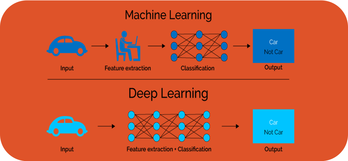
In the introductory video to Deep Learning, we discussed the difference between Machine Learning and Deep Learning. One of the main differences was given by the need of feature extraction. This can be a very time and knowledge demanding task. As we will concentrate on LSTMs in this AI starter kit, fortunately this step is taken care of by the deep learning algorithm itself.

Nevertheless, some data modelling is necessary beforehand. As a first step in the modelling phase, we will prepare the data to serve as input for the LSTM network. When using LSTMs in the time-series domain, one important parameter to pick is the sequence length which is the window for LSTMs to look back in time.

We discussed already in the data understanding video how differently the single variables for a given engine behave and consequently that the time when the degradation becomes visible is different for different engines. Hence, the window size chosen for the training data strongly influences the classification results. In order to model the data for training the algorithm, we first need to reshape the input information. So far, the data consists of the sequential measurements for each of the sensors and settings over time, engine per engine, meaning that one row per cycle and engine is given in the table. This format is however not so suitable for an LSTM model. Therefore, we create a matrix in the format (samples x sequence length x features), where 'samples' is the number of sequences that we will use for model training, ‘sequence length’ is the look back window as discussed before and 'features' is the number of input values of each sequence at each time step. In our case, we selected all sensor values, as well as the 3 settings parameters and the (normalised) current cycle the machine is in at this point.

With the data finally prepared, how can we now actually implement the LSTM architecture? Fortunately, there is no need to start from scratch but there are several open-source tools available that support you when building Deep Learning models. Keras is a deep learning library written in Python. It acts as an interface to the popular tensorflow library. This makes the implementation a lot more feasible.

In the AI Starter Kit though, this is even simpler. Instead of implementing the Deep Learning network yourself, an easy-to-use interface was set up, to adjust the most important variables of the neural network. Once you decide that the parameters specified for building the model are correct, you simply push the “Train model” button at the bottom of the page and the whole implementation and model training is done automatically.

Of course, it is also possible to modify the different parameters directly in the code. For more information on the meaning of each of the settings, you can have a look at the documentation page of Keras. Note that modifying the parameters outside of the scope that is defined in the interactive module can heavily influence the training time and the classification quality. So now it’s time to build your own deep learning model.

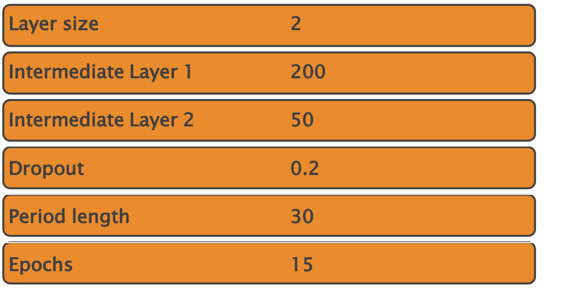
First of all, select the number of intermediate or so-called ‘hidden’ layers. For this first experiment, we select one single intermediate layer only. We set its size to 30 neurons. This corresponds to a rather small network but will be sufficient for a first test. As discussed, we need to decide on the size of the look back window as well. In this first test, we will use a sequence length of 50 cycles. Furthermore, we add a dropout layer after each LSTM layer. The dropout consists in randomly setting a fraction rate of neurons to 0 at each update during training time. This helps preventing overfitting. We choose a value of 0.2 for this first experiment. Finally, we need to select the number of epochs to train. The epochs define the number of times to iterate over the training data arrays. The aim is that the model improves during each training epoch. In general, the more epochs, the better the results until we reach the given model's limit. Here, we will use 15 epochs. This model can now be trained.

Now that we have a trained model, we can evaluate its performance. We will first evaluate it on the training data and subsequently on the test data. If both evaluations result in approximately the same score, this gives an indication that the model is generalizable to unseen datasets and thus not overfitting on the training data. In the interface, we switch to the tab Evaluation on the top of the animation to get more insights into the quality of the trained model. Pushing the button “Evaluate model” will lead to the evaluation of the last trained model.

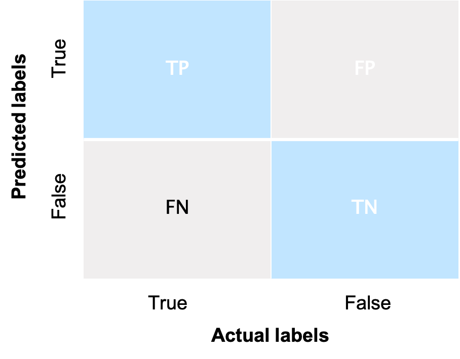
Depending on the use case, different evaluation metrics can be important. Therefore, we will on the one hand evaluate the model in function of accuracy, which measures the fraction of all instances that are correctly categorized. More formally, it is the ratio of the number of correct classifications to the total number of correct or incorrect classifications. On the other hand, we also show the so-called confusion matrix. The confusion matrix shows that the model is able to correctly classify that a specific engine is not going to fail within N cycles for almost all of the more than 12,000 samples. Vice versa, the model is able to correctly classify for almost all of the more than 3000 cases that a specific engine is going to fail within N cycles.

In the summary table at the bottom of the page, several additional metrics are shown. Take your time to go through them once you run these experiments yourself. Note that this evaluation is performed on the training data. In order to evaluate the model against the unknown data, we continue to the next tab in the interface. In this case, the same evaluation as before is performed but on the test data. Also here, the results are promising.

Now run an experiment yourself. For this, chose the following parameters and rerun the pipeline while pausing the video.

Did it work properly? Congratulations! The only differences between the two experiments are the number of layers and their corresponding sizes. Which difference do you observe? Compare the results in the tables in both tabs - evaluation and testing. When comparing the two models, which one would you use and why?

We hope that you have gained more insights in the key factors that influence the quality of a deep neural network and are familiar now with the usage of the interface. We suggest that you try different combinations of settings and think about in which way they influence the quality of the model.

In the next video, we will summarize the key take away messages and provide you with a number of suggestions for additional experiments to gain additional insights.